import time
import tensorflow as tf
config = tf.ConfigProto()
config.gpu_options.allow_growth = True
tf.enable_eager_execution(config=config)
import os
import glob
import numpy as np
from molmod.io import FCHKFile # https://molmod.github.io/molmod/reference/io.html#module-molmod.io.fchk
import multiprocessing

import seaborn as sns
import matplotlib
from matplotlib import pyplot as plt
from scipy.linalg import block_diag

import sys
sys.path.append("../../../")
import tfani
import tfani.aev as AEV

%matplotlib inline

H_fchk = '../HCON/h.fchk'
H_Atom = FCHKFile(H_fchk, ignore_errors=True)
C_fchk = '../HCON/c.fchk'
C_Atom = FCHKFile(C_fchk, ignore_errors=True)
O_fchk = '../HCON/o.fchk'
O_Atom = FCHKFile(O_fchk, ignore_errors=True)
N_fchk = '../HCON/n.fchk'
N_Atom = FCHKFile(N_fchk, ignore_errors=True)
HCNO=[H_Atom, C_Atom, N_Atom, O_Atom]
HCNO_list=['H_Atom', 'C_Atom', 'N_Atom', 'O_Atom']
HCNO_Atom_MO = {}
HCNO_Atom_MO.clear()
self_MO_energies = []
base_HCNO_densities = []
for i in range(len(HCNO)):
    a = HCNO[i]
    coordinates = a.fields['Current cartesian coordinates'] #Bohr
    coordinates = coordinates * 0.529177249 #Angstrom
    species = a.fields['Atomic numbers']
    nuclear_charge = a.fields['Nuclear charges']
    energy = a.fields['SCF Energy'] #Hartree
    MO = a.fields['Alpha Orbital Energies']
    MO_co = a.fields['Alpha MO coefficients']
    density = np.reshape(MO_co, [int(np.sqrt(MO_co.shape[0])), -1])
    base_HCNO_densities.append(density) 
    dipole = a.fields['Dipole Moment']
    num_e = a.fields['Number of electrons']
    print(num_e)
    LUMO = MO[num_e//2]
    HOMO = MO[num_e//2 - 1]
    HCNO_Atom_MO[HCNO_list[i]] = MO
    self_MO_energies.append(MO)
base_HCNO_densities[0].shape

1
6
7
8

/home/richard/program/anaconda3/envs/tf/lib/python3.6/site-packages/molmod/utils.py:228: FutureWarning: Conversion of the second argument of issubdtype from `int` to `np.signedinteger` is deprecated. In future, it will be treated as `np.int64 == np.dtype(int).type`.
  if not np.issubdtype(value.dtype, self.npdtype):
/home/richard/program/anaconda3/envs/tf/lib/python3.6/site-packages/molmod/utils.py:228: FutureWarning: Conversion of the second argument of issubdtype from `float` to `np.floating` is deprecated. In future, it will be treated as `np.float64 == np.dtype(float).type`.
  if not np.issubdtype(value.dtype, self.npdtype):

(2, 2)

print(self_MO_energies[1])
print(self_MO_energies[2])

[-11.333093    -0.82017852  -0.42928032  -0.42928032   0.05473185
   0.70762861   0.70762861   0.74125872   0.78768432   1.90179465
   1.90179465   1.93415807   1.93415807   1.94656579   4.15821066]
[-15.6773628   -1.15895223  -0.56781125  -0.56781125  -0.56781125
   0.80530464   0.84474176   0.84474176   0.84474176   1.90664544
   1.90664544   1.90664544   1.90664544   1.90664544   3.54280788]

plt.figure(figsize=(16,2))

with sns.axes_style("white"):
    ax = sns.heatmap(base_HCNO_densities[0], square=True, linewidths=.5,  cmap="YlGnBu", annot=True, center=0.)
    plt.xlabel('wavefunction', fontsize=14)
    plt.ylabel('Coeffients', fontsize=14)
    plt.show()

def plot_MO(ground_true, pred, i, hide_padding=True):

    ground_true_data = ground_true[i]
    pred_data = pred[i]

    x = np.linspace(1, len(ground_true_data), num=len(ground_true_data))    
    diff = np.absolute(ground_true_data - pred_data)
    diff_large_idx = np.squeeze(np.argwhere(diff>0.024))
    diff_large_data = np.take(ground_true_data, diff_large_idx)

    plt.figure(figsize=(18,10))

    # plot diff > 0.04
    plt.plot(diff_large_idx + 1, diff_large_data, label='diff > 0.024 hartree | 15.04 kcal/mol ({} points)'.format(len(diff_large_idx)), 
             marker='x', linestyle = 'None', markersize=10, markeredgewidth=1, color='magenta')    

    # plot ground ture
    plt.plot(x, ground_true_data, label='ground true', marker='.', linestyle = '-', markersize=10, 
             markeredgewidth=1, color='r')

    # plot pred
    plt.plot(x, pred_data, label='prediction', marker='.', linestyle = '-', markersize=10, 
             markeredgewidth=1, color='g')

    # title and label
    plt.title('Using ANI to Predict Molecular Orbitals',  fontsize=18)
    plt.xlabel('Molecular Orbitals', fontsize=18)
    plt.ylabel('MO Energy / hartree', fontsize=18)
    plt.legend(frameon=False, fontsize=16)
    plt.ylim(-20, 6)
    plt.show()

plt.figure(figsize=(16,10))

with sns.axes_style("white"):
    ax = sns.heatmap(base_HCNO_densities[2], square=True, linewidths=.5,  cmap="YlGnBu", annot=True, center=0.)
    plt.xlabel('wavefunction', fontsize=14)
    plt.ylabel('Coeffients', fontsize=14)
    plt.show()

# plt.figure(figsize=(16,10))

# with sns.axes_style("white"):
#     ax = sns.heatmap(base_HCNO_densities[1]-base_HCNO_densities[2], square=True, linewidths=.5,  cmap="YlGnBu", annot=True, center=0.)
#     plt.xlabel('wavefunction', fontsize=14)
#     plt.ylabel('Coeffients', fontsize=14)
#     plt.show()

# C2NH5
tmp = FCHKFile('./gdb11_s03-0000024_0221.fchk', ignore_errors=True)
a = tmp
species = a.fields['Atomic numbers']
MO = a.fields['Alpha Orbital Energies']
MO_co = a.fields['Alpha MO coefficients']
density = np.reshape(MO_co, [int(np.sqrt(MO_co.shape[0])), -1])
num_e = a.fields['Number of electrons']
coordinates = a.fields['Current cartesian coordinates'] #Bohr
coordinates = coordinates * 0.529177249 #Angstrom
coordinates = np.reshape(coordinates, [-1, 3])

plt.figure(figsize=(16,10))
with sns.axes_style("white"):
    ax = sns.heatmap(density, square=True, linewidths=.0,  cmap="YlGnBu", annot=False, center=0., cbar=False)
    plt.vlines(x=15, ymin=0, ymax=55, colors='darkgray')
    plt.vlines(x=30, ymin=0, ymax=55, colors='darkgray')
    plt.vlines(x=45, ymin=0, ymax=55, colors='darkgray')
    plt.vlines(x=47, ymin=0, ymax=55, colors='darkgray')
    plt.vlines(x=49, ymin=0, ymax=55, colors='darkgray')
    plt.vlines(x=51, ymin=0, ymax=55, colors='darkgray')
    plt.vlines(x=53, ymin=0, ymax=55, colors='darkgray')
    for i in range(55):
        plt.hlines(y=i, xmin=0, xmax=55)
    plt.xlabel('wavefunction', fontsize=14)
    plt.ylabel('Coeffients', fontsize=14)
    plt.show()

pred = []
pred.append(self_MO_energies[1])
pred.append(self_MO_energies[1])
pred.append(self_MO_energies[2])
pred.append(self_MO_energies[0])
pred.append(self_MO_energies[0])
pred.append(self_MO_energies[0])
pred.append(self_MO_energies[0])
pred.append(self_MO_energies[0])
pred = np.concatenate(pred, axis=0)

plot_MO([MO], [pred], 0)

idx = np.argsort(pred)
sort_pred = np.take(pred, idx)

plot_MO([MO], [sort_pred], 0)

NCCHHHHH = block_diag(base_HCNO_densities[1], base_HCNO_densities[1], base_HCNO_densities[2], base_HCNO_densities[0],
                      base_HCNO_densities[0], base_HCNO_densities[0], base_HCNO_densities[0], base_HCNO_densities[0])

plt.figure(figsize=(16,10))

with sns.axes_style("white"):
    ax = sns.heatmap(NCCHHHHH, square=True, linewidths=.0,  cmap="YlGnBu", annot=False, center=0.)
    plt.hlines(y=15, xmin=0, xmax=30)
    plt.vlines(x=15, ymin=0, ymax=30)
    plt.hlines(y=30, xmin=15, xmax=45)
    plt.vlines(x=30, ymin=15, ymax=45)
    plt.hlines(y=45, xmin=30, xmax=55)
    plt.vlines(x=45, ymin=30, ymax=55)
    plt.xlabel('wavefunction', fontsize=14)
    plt.ylabel('Coeffients', fontsize=14)
    plt.show()

sort_NCCHHHHH = np.take(NCCHHHHH, idx, axis=0)
# sort_NCCHHHHH = np.take(np.transpose(NCCHHHHH), idx, axis=0)
# sort_NCCHHHHH = np.transpose(sort_NCCHHHHH)

plt.figure(figsize=(16,10))

with sns.axes_style("white"):
    ax = sns.heatmap(sort_NCCHHHHH, square=True, linewidths=.0,  cmap="YlGnBu", annot=False, center=0., cbar=False)
    plt.vlines(x=15, ymin=0, ymax=55, colors='darkgray')
    plt.vlines(x=30, ymin=0, ymax=55, colors='darkgray')
    plt.vlines(x=45, ymin=0, ymax=55, colors='darkgray')
    plt.vlines(x=47, ymin=0, ymax=55, colors='darkgray')
    plt.vlines(x=49, ymin=0, ymax=55, colors='darkgray')
    plt.vlines(x=51, ymin=0, ymax=55, colors='darkgray')
    plt.vlines(x=53, ymin=0, ymax=55, colors='darkgray')
    for i in range(55):
        plt.hlines(y=i, xmin=0, xmax=55)
    plt.xlabel('wavefunction', fontsize=14)
    plt.ylabel('Coeffients', fontsize=14)
    plt.show()

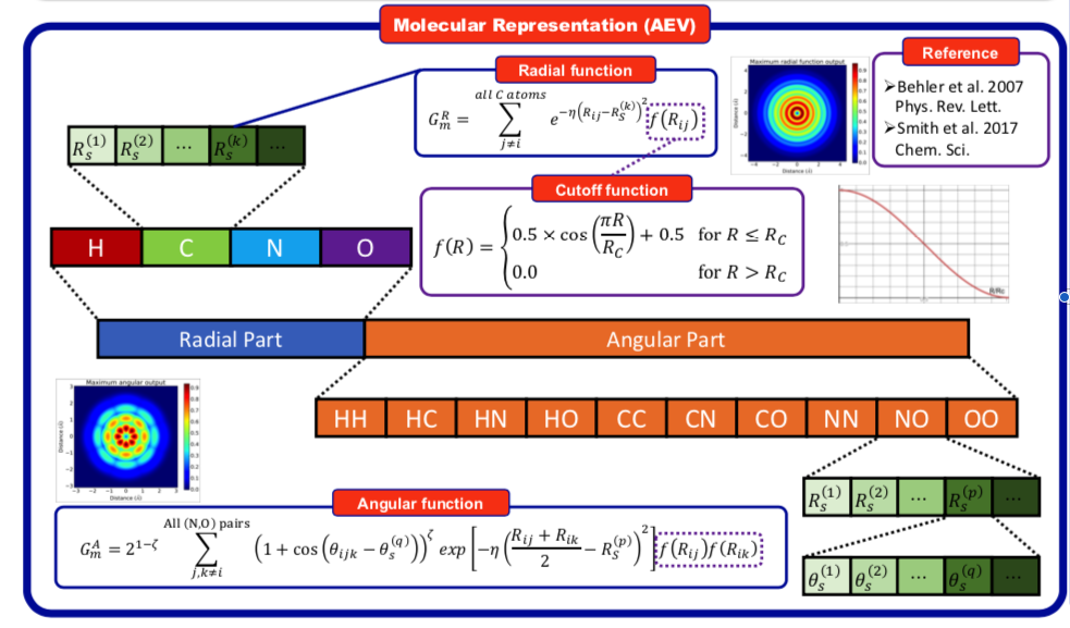
# constants
constants = {
    'Rcr': 5.2000e+00,
    'Rca': 3.5000e+00,
    'EtaR': [1.6000000e+01],
    'ShfR': [9.0000000e-01,1.1687500e+00,1.4375000e+00,1.7062500e+00,1.9750000e+00,
             2.2437500e+00,2.5125000e+00,2.7812500e+00,3.0500000e+00,3.3187500e+00,
             3.5875000e+00,3.8562500e+00,4.1250000e+00,4.3937500e+00,4.6625000e+00,4.9312500e+00],
    'Zeta': [3.2000000e+01],
    'ShfZ': [1.9634954e-01,5.8904862e-01,9.8174770e-01,1.3744468e+00,1.7671459e+00,
             2.1598449e+00,2.5525440e+00,2.9452431e+00],
    'EtaA': [8.0000000e+00],
    'ShfA': [9.0000000e-01,1.5500000e+00,2.2000000e+00,2.8500000e+00],
    'num_species': 4}

_, aev = AEV.AEVComputer(**constants)(([tf.cast(species, tf.int64)], [tf.cast(coordinates, tf.float32)]))
aev = tf.squeeze(aev, axis=0)

print(species)

[<tf.Tensor: id=598, shape=(8,), dtype=int64, numpy=array([6, 6, 7, 1, 1, 1, 1, 1])>]

plt.figure(figsize=(60,30))

with sns.axes_style("white"):
    ax = sns.heatmap(aev, square=True, linewidths=.0,  cmap="YlGnBu", annot=False, center=0., cbar=False)
    plt.xlabel('AEV', fontsize=14)
    plt.ylabel('Atom', fontsize=14)
    plt.show()

aev

<tf.Tensor: id=3957, shape=(8, 384), dtype=float32, numpy=
array([[0., 0., 0., ..., 0., 0., 0.],
       [0., 0., 0., ..., 0., 0., 0.],
       [0., 0., 0., ..., 0., 0., 0.],
       ...,
       [0., 0., 0., ..., 0., 0., 0.],
       [0., 0., 0., ..., 0., 0., 0.],
       [0., 0., 0., ..., 0., 0., 0.]], dtype=float32)>

Think about how to improve AEV?